For this purpose, we will search for all records containing the disaccharide 4-O-β-D-galactopyranosyl-2-amino-β-D-glucopyranose (both N-acetylated and non-N-acetylated) OR 4-O-β-D-galactopyranosyl-β-D-glucopyranose for which NMR data are deposited in the CSDB.
|
|
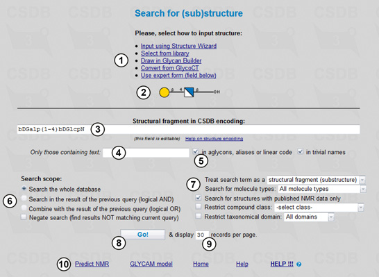
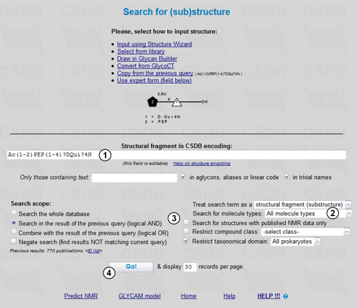
To perform a search, first of all we should select the search type in the main menu of BCSDB. The problem specified requires the (Sub)structure search, the form for which is shown in Fig. 1.1. Here we fill in search terms (3,4), select a scope (6), ) and additional parameters (7), and run the query (8). The structural fragment being searched is previewed (2) in the graphic form according to the Essentials of Glycobiology v. 3 (SNFG standard), which extends the format known as 'CFG notation'. If you edit the search term manually and your query cannot be parsed, area (2) displays the parsing errors.
Every search form except ID search has a selector identifying the search scope (6). This feature allows refining the queries by their intersection or combination with queries of the same or different type. Search in the result of the previous query intersects the current and previous queries (logical AND), whereas Combine with the result of the previous query unites the current and previous queries (logical OR). Negate search negates the current query (logical NOT) and can be used both to get all the results present in the database except those that match the current search criteria and to exclude the results matching the current search criteria from the ones of the previous query (when the check box Search in the result of the previous query is checked).
A number of found records displayed per page can be specified (9). Links to additional CSDB tools (10) are also available.
To query the database for structures, we should enter a structure of interest into the search field (3). CSDB allows several ways to do that (1):
The disaccharides chosen for this example are simple and can be created without using the CSDB linear code. For exemplary purposes, we will use Glycan Builder to build 4-O-β-D-galactopyranosyl-2-amino-β-D-glucopyranose.
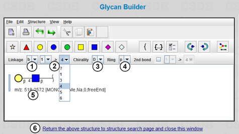 |
Follow the link Draw in Glycan Builder(1) (Fig. 1.1), and the Glycan Builder will open in a new window (Fig. 1.2). This plugin requires Java environment installed on your computer. The menu View allows choosing the view mode of the fragment being drawn: Essentials of Glycobiology v.2 ("CFG notation"); UOXF (Oxford) notation; or text only. You can link residues by selecting them from the menu; anomeric configuration (beta, alpha, or unknown) (1), chirality (D, L, or unknown) (3), ring size (pyranose, furanose, open, or unknown) (4), and a linkage between the residues (carbon atom numbers of the donor and the acceptor) (2) can be specified. The resulting structure is shown in field (5). Pressing link (6) returns the structure to the (Sub)structure search page and closes the Glycan Builder.
The menu contains no GlcN residue; therefore, we will use widespread GlcNAc residue (which becomes two residues in the CSDB notation, GlcN and Ac), and the returned structure will be 4-O-β-D-galactopyranosyl-2-deoxy-2-acetamido-β-D-glucopyranose written in the CSDB encoding: bDGalp(1-4)[Ac(1-2)]bDGlcpN. To get the target structure, we must "deacetylate" the N-acetylglucosamine residue, i.e. manually delete the [Ac(1-2)] part from the structure field. The page with the resulting structure (3) and its visualization in the EOG3 format (2) is shown in Fig. 1.1. This query will find structures with non-acetylated, as well as with acetylated amino groups.
We will conduct the search with the following restrictions: the search will include molecules of all types (monomers, oligomers, repeating units, cyclic compounds etc.) (7) and will be conducted through the whole database (6), with no additional restrictions on text content (4) present in aglycons, aliases, linear code or trivial names (5), structure completeness, or compound class (7). Since we are interested only in the records containing the NMR data, the Search for structures with published NMR data only checkbox should be checked (7).
Pressing the Go! button (8) starts the search.
 |
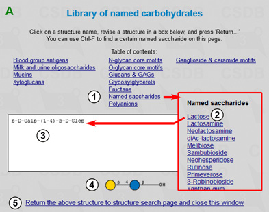
The search results in 44 structures containing the target fragment. Now we will extend our query by searching for all the structures containing the 4-O-β-D-galactopyranosyl-β-D-glucopyranose disaccharide. By pressing the New query link (at the bottom of the result page) or through the main menu we return to the Search for (sub)structure form. Since 4-O-β-D-galactopyranosyl-β-D-glucopyranose is a widespread named disaccharide "lactose", we can select it from the structure library by clicking Select from library, which opens a new window (Fig. 1.3A). Here we choose lactose (2) from Named saccharides (1), and the corresponding structure is previewed in the SweetDB pseudo-graphic (3) or in the SNFG graphic (4) form. Pressing (5) returns the structure to the structure search page and closes the library.
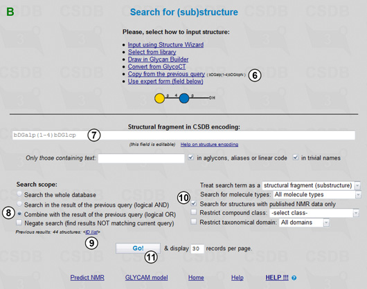
The query form with the lactose disaccharide, bDGalp(1-4)bDGlcp (7), is shown in Fig. 1.3B. Note that we could also copy and manually edit the structure from the previous structural query (6).
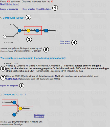 |
Now we are ready for the final step - combining the results of both queries. By choosing Combine with the result of the previous query (8) (the number of these results is shown on the page together with the link to their ID list (9)) we define the search scope as the database records matching the current structural fragment, 4-O-β-D-galactopyranosyl-β-D-glucopyranose, plus the records matching the previous one, 4-O-β-D-galactopyranosyl-2-amino-β-D-glucopyranose, with published NMR data only (10). Pressing (11) starts the search. The combined result includes 109 structures containing any of the target disaccharides for which NMR data are present in the database (Fig. 1.4).
On the result page, all compounds are displayed in the collapsed form (Fig. 1.4) showing the most important data only. The header contains the number of structures found, a link to the next page of results, a link expanding all records, and a switch between graphic (SNFG) and pseudo-graphic (SWEET-DB) representations of the structures (1). (1). For each compound found, its compound ID (2), structure (3), visualization tools (4), structure type and compound class (if present) (5) are displayed. Each compound has a list of publications in which it was published (6); in the depicted case it contains only one item. The combination of an article and a compound is called a record and has a persistent CSDB record ID. To access the record, press link (7) that retrieves all the record data, such as NMR spectra etc. Link (8) expands the entry showing more data associated with the compound.
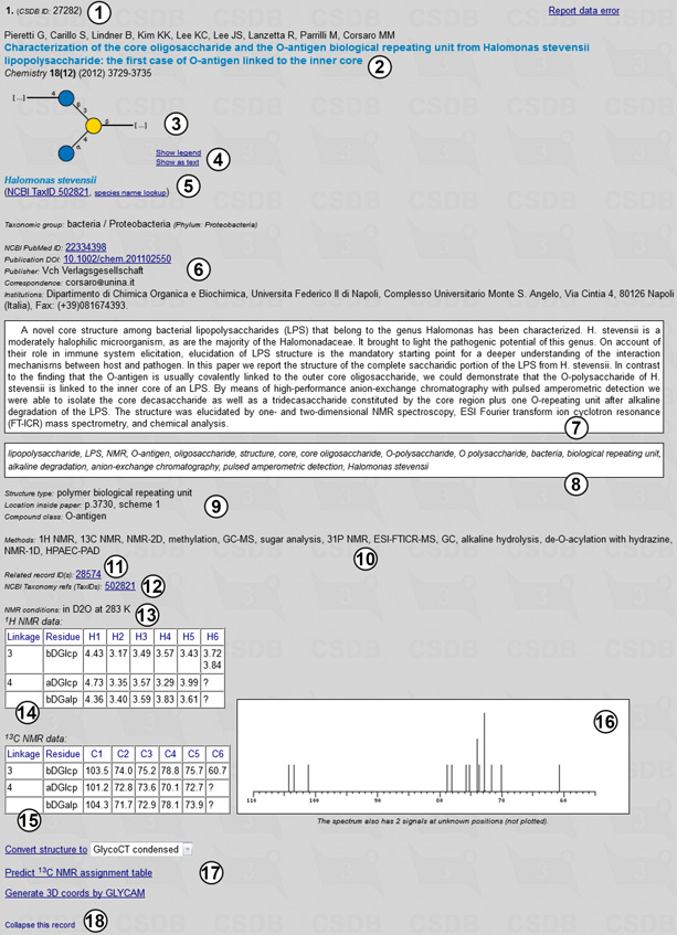 |
Fig. 1.5 shows record 27282 for the second compound from Fig. 1.4 in the expanded form. The following information is provided: a CSDB ID for the record (1) (it can be used later to access a certain record by its ID); authors and imprint of the paper containing the compound (2); a graphic (SNFG) or pseudo-graphic (SweetDB similar to the extended IUPAC) representation of the structure (3,4); taxonomic data on the organism(s) from which this compound was obtained in this publication, together with taxon renaming information and links to the NCBI Taxonomy database by name or TaxID (5,12); links to NCBI PubMed and DOI resources, as well as information on publisher, affiliation and contacts of the authors (6); abstract (7) and keywords (8) of the paper; structure type and compound class, location of the structure in the paper (9); methods used in the paper (10); links to the related records within CSDB and other databases if available (11); NMR conditions (temperature and solvent) (13), 1H NMR (14) and 13C NMR (15) signal assignment tables of the compound, as well as an overview of its 13C NMR spectrum (16); and links to additional CSDB tools (17). Link (18) collapses the expanded record.
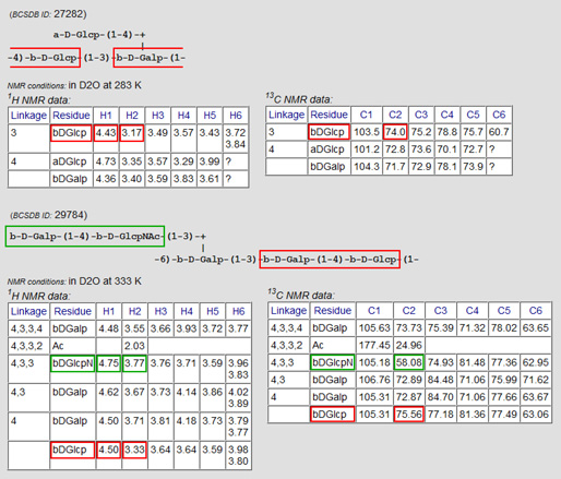 |
To see an effect of the presence of amino group on chemical shifts, we should look at the NMR tables for the compounds found. Fig. 1.6 shows NMR data for BCSDB records 27282 and 29784, the former of which contains 4-O-β-D-galactopyranosyl-β-D-glucopyranose and the latter of which contains both 4-O-β-D-galactopyranosyl-β-D-glucopyranose and 4-O-β-D-galactopyranosyl-2-amino-β-D-glucopyranose. Chemical shifts that differ significantly between the two structures are shown in red (glucose) and green (glucosamine). The highlighted values of chemical shifts account for alpha- and beta-amination effects of galactose within lactose.
This problem can be solved by using the Composition search available from the main menu of CSDB. The search query is shown in Fig.2.1.
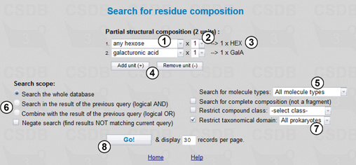 |
Here we can select a partial structural composition for our search. In Fig. 2.1, the composition includes two units, one unspecified hexose and one galacturonic acid. Drop-down list (1) allows selection of a residue from the list of the most common cases. If a residue of interest is missing from the list, select the first (or the last) entry COMPLETE LIST to look through all residues present in the database. Drop-down list (2) indicates the minimal number of the residue instances in the structures to search for, which is also reflected in the composition preview area (3). Buttons (4) add or remove residues from the composition.
In this query, we will include all types of molecules stored in CSDB (5), and the search will be carried out through the whole database (6), with no restriction on the composition completeness or compound class. Since we are interested in bacterial glycans in this example, we limit the result to the structures associated with Prokaryotes by choosing the taxonomical domain restriction of All Prokaryotes (7). The query will return all structures containing at least one hexose residue and one galacturonic acid residue. Pressing the Go! button (8) starts the search resulting in 738 compounds.
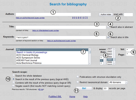 |
Now we will refine the results by choosing only structures from the papers published after 2005 and containing various word forms of the term antigen in the article title or keyword list. For this purpose, we select Bibliography from the main menu (Fig. 2.2).
In the Bibliography search mode, we can compose queries using imprint and meta-data of publications. We can specify authors (1), directly or from index (2), full or partial title (3) (with or without abstract; see search also in abstract checkbox (4)), keywords (5) (with or without title terms; see search also in title checkbox (6)); select a journal from list (7) and specify the publication year (8) (exact (=), newer than (>), or older than (<)), as well as volume or pages (9). Term fields (1), (3), and (5) support queries with logical operations, term grouping and wildcards; specific national symbols are available (1). The search is case-sensitive and accent-independent.
To search for papers published after 2005 and containing keywords or titles which include antigen, we enter *antigen* in field (5) and check checkbox (6). As the star character is a wildcard for any number of characters, this query will process all terms like antigens, antigenic, O-antigen, etc. To start, we select the year span newer than 2005 (8), check Search in the results of the previous query (10), and press the Go! button (11).
The results include 73 publications. One of them is shown in Fig. 2.3.
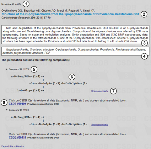 |
In contrast to the (Sub)structure search, which returns compounds, the Bibliography search results in a list of publications. In the case of our combined query, each of these publications includes one or several structures at least one of which matches the composition query and contains at least one galacturonic acid residue and one more hexose residue. For each publication, its article ID (1), imprint data (2), abstract (3) and keywords (4) are shown, and the list of compounds present in the paper is displayed, with the corresponding compound ID (5), representation of the structure in the SNFG or SweetDB format (6), and an organism from which the compound was extracted, as well as a link to retrieve all the data (8) available in the record. Switch (7) allows selecting the structure representation format (graphic vs. psudographic). In Fig 2.3 the structure display format was chosen as SweetDB (pseudograpic).
Fig. 2.3 shows that in this example all the compounds present in the paper match the initial composition query (1 x HEX + 1 x GalA + ...). However, if at least one of the structures in the paper matches the query, such paper is included into the search results, and therefore compounds from the same paper with composition different from that specified are also shown.
To search for compounds obtained from organisms belonging to a certain genus we will use the Taxonomy search from the main menu (Fig. 3.1).
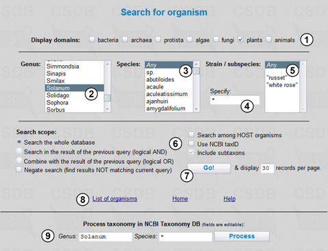 |
The Display groups option (1) allows specifying a target domain(s) of organisms; in our case it is plants only. By using lists of genera (2) and species (3) we specify Solanum as genus and Any as species implying that all species belonging to this genus will be searched for, including Solanum organisms with undetermined species. Fields (4) and (5) specify subspecies by selection from those available for the current genus (5) or by direct input of a character pattern (4) (fragment of name or * for no limitations). The search will be conducted through the whole database, with taxonomic children included (6): all organisms belonging to the specified group and its subgroups will be returned; if we use the selection lists, the taxonomic children are always included. Other available options are Search among HOST organisms (returns an organism specified and structures found in microorganisms or parasites infecting the target organism or extracted from it) and Use NCBI Tax ID (the taxon selection lists disappear, and we can indicate a position of taxon on the tree of life by its NCBI TaxID). We can access the full list of organisms present in the database (8) or process the taxonomic request in the NCBI Taxonomy database (9) (retrieves taxonomic lineage and other data for the genus and species specified). Pressing button (7) starts the search resulting in 48 organisms.
To find only those compounds from the Solanum genus that contain the steroidal alkaloid solanidine, we will use the (Sub)structure search (Fig. 3.2).
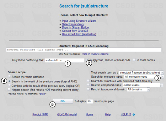 |
Solanidine is not a carbohydrate and it has no reserved residue name in CSDB; therefore, it can be present only as aglycon or inside the alias explanation. To search through aglycons and aliases, we will enter solanidine in field (1), with the in aglycons, aliases or linear code checkbox checked (2). The search will include all molecule types (3) and will be carried out in the results of the previous query (4). Pressing button (5) starts the search resulting in 16 compounds each of which contains solanidine as aglycon and is extracted from the Solanum plants. The layout of the result page is close to that described in Example 1.
This problem addresses residues with the specified feature in the NMR spectra. However, an overabundance of NMR data for structures containing 3-deoxy-D-manno-oct-2-ulosonic acid (Kdo) would obscure the results, so we will search only for those compounds, which do NOT contain octoses. We will start this search from the NMR signals in the CSDB menu (Fig. 4.1).
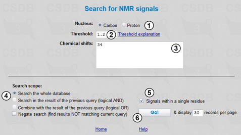 |
Here we specify the nucleus (1) and chemical shift(s) (3) (numerals and decimal dot are allowed). The signals can be separated with spaces or new-line characters; sorting is not required. The Threshold field (2) determines how accurate the correspondence of signals to the specified values should be. It filters the result by spectra similarity returning only those with similarity higher than the threshold. To calculate the similarity between the specified and stored spectra, the CSDB engine forms all possible subspectra of the larger NMR spectrum with the number of signals equal to that found in the smaller spectrum, and the best-fitting subspectrum is used to calculate the similarity value. Similarity is an inverse average deviation between the signals normalized by the number of signals in the smaller spectrum. 0 is reserved for no similarity, and 1000 is for full similarity (exact match of chemical shifts). Good similarity values are 1 and above for carbon spectra and 5 and above for proton spectra.
We will carry the search out through the whole database (4). Note that the Signals within a single residue checkbox is checked by default (5), but since we are searching for a single signal it is of no importance in our case. Pressing button (6) starts the search resulting in 133 compounds sorted by spectra similarity.
Fig. 4.2 shows one of the found compounds and its NMR spectrum.
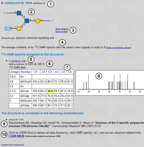 |
For each compound found, its ID (1), graphic or pseudo-graphic representation of the structure (2), visualization tools (3) and structure type are displayed. The average similarity between the 13C NMR spectra of this compound and the search term is shown (4), together with the spectrum itself (7,8), experimental conditions (6), and a link to the paper in which it was published (5). Signal matching the search term are highlighted in yellow. The information about the paper is also given (9), and the link to the full data on the record is present, together with the organism from which this compound was extracted (10).
To refine the search results to the compounds that contain no octose residues, we will use the Composition search mode (Fig. 4.3).
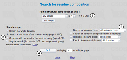 |
We choose a partial structural composition of one unit, octose (1), and include all molecule types (2). To perform logical exclusion (AND NOT operation) we define the search scope as Search in the result of the previous query and check the Negate search checkbox (3). Pressing the Go! button (4) will find all compounds, which contain no octose residues and spectra of which contain at least one signal close to 34 ppm. The final result list includes 71 compounds in which this signal originates from non-sugar residues and deoxy-sugars other than Kdo (3-deoxy-D-manno-oct-2-ulosonic acid), Ko (D-glycero-D-talo-oct-2-ulosonic acid) or other octoses.
Since every search form provides more than one search criteria, you should be careful about usage of negation. For example, specifying the negation together with two criteria (octose-contaning and Prokaryote domain) will hardly make sense because [NOT (octose-containing AND prokaryotic)] is the same boolean logic as [(NOT octose-containing) OR (NOT prokaryotic)]. If you wish to filter the results to prokaryotic structures only and you still need a negation in the complex query, you should use the structure search once more, specify structure=ANY and domain=Prokaryotes, and intersect it with the previous results.
First we will find papers written by Knirel or Shashkov AS using the Bibliography search mode (Fig. 5.1).
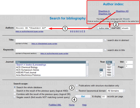 |
The author query Knirel OR "Shashkov AS" (1) will find all papers authors of which include at least one of the names specified, Knirel (any initials) or Shashkov AS (explicit initials). To insert a specific author name and initials from the index, type the starting characters in field (2), press Author index, and select an author. Quotes allow inclusion of blank spaces in the search term, e.g. the author last name and initials. The author index (2) can be used for picking up the author names. You should type at least two characters to display the list of author names starting with these characters. The search will be carried out through the whole database (3). For other bibliography search options available, see Example 2. Pressing the Go! button (4) starts the search resulting in 770 publications.
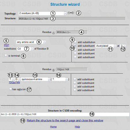 |
To find among these publications only those with structures containing quinovose-4-amine amidated by any N-acetylated amino acid, we will use the (Sub)structure search mode and will enter the disaccharide using the structure wizard (Fig. 5.2).
The usage of the structure wizard does not require special knowledge except for the general nomenclature of carbohydrates. First of all, we select a suitable topology from drop-down list (1) (topologies of up to four residues are supported), and the graphic representation of the selected topology is displayed (2). When the topology is selected, the corresponding number of residue sections appears below (two in our case). Structure (3) shows the target structure in the IUPAC condensed form. Residue section header (4) shows the position of this residue within the selected topology (e.g. Residue A) and the residue name with configurations and substitutions.
The left part of the residue section includes the drop-down list of residue names (6,15). Only the most common residues are listed; if a residue of interest is missing, select the first (or the last) entry complete list. In our case, the superclass any amino acid is selected for Residue A (6), and quinovose-4-amine is selected for residue B (15). If applicable to the selected residue, configuration options are available: anomeric configuration (alpha, beta, or ? for any) (13); absolute configuration (D, L, R, S, or ? for any) (14); and residue ring form: pyranose, furanose, open-chain, alditol, or ? for any form (16). Link (5) shows the resulting residue name without substitutions and leads to the complete list window. Linkage control (7) specifies the position in the acceptor residue substituted by the current residue (in this case, C4, which means that Residue A is linked to C4 of Residue B). The position of the current residue by which it substitutes the acceptor is C1 for aldo-sugars and non-sugar residues, and C2 for keto-sugars. The linkage control does not apply to the residue at the reducing end of the fragment. The is terminal checkbox (8) indicates that this residue should not be substituted by anything except monovalent substituents and is visible only for residues occupying terminal positions in the selected topology. The residue at the reducing end (in the last residue section, or, in this case, Residue B) has the aglycon checkbox (17) and a corresponding drop-down list (hidden in Fig. 5.2) allowing to select an aglycon.
The right half of the residue section allows adding substituents. Usually this feature is used to indicate the position of attachment of another repeating unit (9) to the leftmost residue in the polymer repeat, or positions of monovalent substituents like acetyl groups (10-12). Thus, the amino acid residue in our structure is acetylated (11) at position 2 (12).
 |
The constructed structure in the CSDB encoding is displayed at the bottom of the page (18). Pressing the Return the structure to the structure search page link (19) transfers the query into the (Sub)structure search form (Fig. 5.3) and closes the wizard.
Fig. 5.3 shows the (Sub)structure search form with the disaccharide fragment (1) returned by the structure wizard. The search will include all molecule types (2) and will be conducted in the results of the previous query (3). Pressing the Go! button (4) results in 11 compounds containing the specified disaccharide published in the papers written by Knirel or Shashkov AS. The layout of results is similar to those in Example 1.
This simple query demonstrates how the Search for complete composition option can be used. We will perform the search in the composition search mode. Fig. 6.1 shows the query.
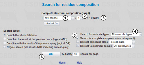 |
To find all structures containing only one nonose monosaccharide, we select the complete structural composition (3): any nonose (1) occurring once within the structure (2). Then we choose all molecule types (4), check the Search for complete composition (not a fragment) checkbox (5), and restrict taxonomical domain to All prokaryotes. Pressing the Go! button (6) returns 7 compounds each of which is a prokaryotic nonose monosaccharide or a prokaryotic nonose homopolymer with or without monovalent modifications.
CSDB contains ca. 8500 NMR spectra recorded in water, facilitating statistical simulation of the NMR data in water solutions. The distribution of solvents vs. records in the current database can be displayed by presing Coverage link (6). The NMR simulation link in Extras from the main menu opens the spectrum simulation form (Fig. 7.1). As the options for structure input (1) and visualization (2) have been described in the previous examples, here we will use the expert form and type the target structure in the CSDB encoding in field (3): aXAbep(1-3)bD6dmanHepp(1-P-1)xDRib-ol.
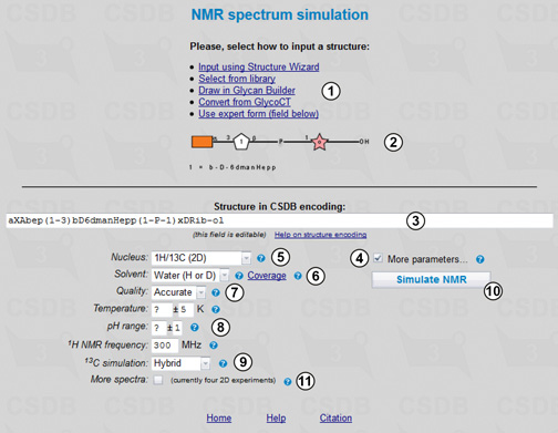 |
By default, only the nucleus (5) and solvent (6) parameters are displayed, however checking More parameters... (4) shows all of them, as in the figure. We will select 1H/13C for nucleus (5) to simulate 1D and 2D NMR spectra, Water as a solvent (6) and use the accurate quality mode (7). There are three modes of simulation, depending on quality vs. speed: fast, accurate (default), and extreme. If you see unpredicted signals (question marks) in the assignment, set this option to higher quality and press button (10) once again. Note that in the extreme quality mode, the calculation may take up to 15 minutes. Together with the solvent, additional simulation parameters (8), such as pH or temperature range, allow limiting the database scope to the data obtained under certain experimental conditions.
For carbon chemical shifts, both empirical and statistical simulation approaches will be employed to obtain a hybrid result (9). The empirical simulation is based on an incremental scheme with steric correction and utilizes internal databases of reference chemical shifts of mono-, di- and trimeric fragments and substitution effects. The algorithm was adopted from the earlier work. The statistical simulation is based on sequential generalization of the atomic surrounding of the predicted atom until enough structurally similar fragments are found in CSDB, with subsequent outlier detection and data averaging (ref. 1, ref. 2). The hybrid approach combines the results of empirical and statistical simulations in accordance with trustworthiness reported by both approaches. It becomes available if the hybrid mode is selected for carbon chemical shifts, and the solvent is water or unrestricted. Proton chemical shifts are always simulated statistically.
Pressing button (10) simulates the NMR spectra (Fig. 7.2).
 |
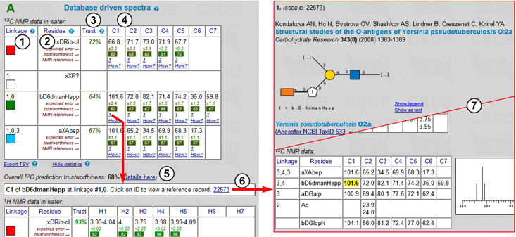
Assignment tables and schematic 13C NMR plots predicted by the three different approaches (empirical, statistical, and hybrid) are displayed. A part of the result page (statistical assignment tables, full output of hybrid approach, and exemplary 2D plots) is shown in Fig. 7.2.
Every residue is represented by a single row in the assignment table. Each row is identified by linkage data (the linkage path to the residue from the oligomer reducing end or from the rightmost residue in the repeating unit of a polymer) (1) and a residue name in the CSDB linear code (2). Every row also contains a color square (in the Linkage column (1)) identifying the color code of signals in the 2D NMR plots. C1..C9 columns (4) list the chemical shifts and supplementary data. In the empirical assignment table (not shown), these data include chemical shifts of unsubstituted residues and substitution effects. Fig. 7.2A shows the the results of the statistical 13C NMR simulation. In the assignment table, there are expected simulation error (in ppm) and trustworthiness metrics (in %) for every signal, the number of database records used to obtain the averaged data and a link to the processing report. Clicking on the number of records below each chemical shift opens a list of references (6). These references allow tracking the source of data to CSDB records and corresponding original publications (7). The data used in simulation are highlighted (X) in these records.
The trust column (3) provides the trustworthiness averaged from all atoms in the residue. Trustworthiness values vary from 0 to 100% and are color-coded (uniformly from poor to good). Overall prediction trustworthiness is shown below the table (5). The correlation between the trustworthiness level and chemical shift calculation accuracy was established by linear regression. It is used to predict the expected simulation error in ppm, which is displayed below each chemical shift.
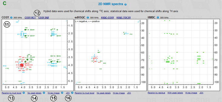
If 1H or 1H/13C was specified as a nucleus, 2D NMR spectra are visualized using the predicted chemical shifts (Fig. 7.2C). Depending on the nucleus and the state of More NMR experiments checkbox, two to eight 2D spectra are plotted. These experiments cover most of proton and carbon spin correlations commonly used in glycobiology (COSY, TOCSY, HSQC, HMBC and derived experiments). NOE correlations are currently not supported. As an example, COSY, edHSQC and HMBC are shown in the figure (11). Links (12) lead to the experiments related to that displayed. Links below the spectrum switch useful display options: color mode, signal labels and image resolution.
The color mode switch (13) determines how the signals are colored; it has two states: signal assigment and trustworthiness level. The former colors all the signals according to the residue color code, as displayed in the first column of the assignment table (exemplified in COSY and edHSQC). The latter colors all the signals in the range from red to green reflecting how accurate the simulation of the signal was (exemplified in HMBC).
The peak label switch (14) hides or shows the numbers beside signals. In the assignment color mode, these numbers correspond to the order of carbon atoms in the structure. The combination of the color (=residue) and the label (=position in a residue) identifies every atom. NMR spectra, which provide non-direct correlations, may have complex labels, including bi-colored ones (e.g. H1/C3) to identify inter-residue cross-peaks. In the trustworthiness color mode, numbers are the trustworthiness metrics. In Fig. 7.2C, HMBC is displayed without labels in the trustworthiness color mode, while COSY and edHSQC are displayed with labels in the assignment color mode.
The Hi-res image link (15) or clicking on a spectrum displays a larger image in a separate window for copy-and-pasting. If some of the signals could not be predicted (they have ? as a chemical shift in the assignment table), they are listed below the spectra in which they should have appeared. The JDX link (16) exports the spectrum in the Jcamp-DX format, which can be opened and further processed in external NMR software, such as MestreLabs MestreNova, ACD/Labs NMR viewer or Bruker TopSpin.
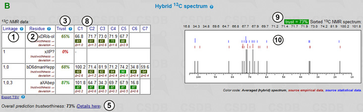 |
Fig. 7.2B shows the results of 13C simulation via the hybrid approach. It implies heuristic mixing of data from both approaches according to their deviation, trustworthiness, dataset size and other parameters. As it benefits from both simulation methods, it usually provides most accurate results. The hybrid supplementary data contain the trustworthiness metrics and inter-approach deviation (Δ) for each atom. The reference data from both approaches (red marks = empirical, blue marks = statistical) are added to the spectrum plot (10). The header reports the overall trustworthiness metrics and lists all signals in sorted order (9) for copy-and-pasting.
For more data on NMR spectra simulation algorithms utilized, including evaluation of accuracy and trustworthiness of predictions, and hybridization details, please refer to dedicated publications. A brief review is also given in the Help.
In our example, both empirical (not shown) and statistical (Fig. 7.2A) approaches reported relatively low trustworthiness (60%) for C1 of β-6-deoxy-mannoheptopyranose. Statistical data were taken from a single database record. By clicking on 1 (the number of used records) in the C1 column in the bD6dmanHepp row, we can explore where the data came from and see that the structure has undergone strong permutations during the generalization process, which explains the low trustworthiness metrics. The list of permutations applied to fit records present in the database is individual for each atom and available under the How? link.
This problem can be solved by using the NMR-based structure elucidation tool available from Extras in the main menu. Fig. 8.1 shows the input form. Assume that we know the monomeric composition from chromatographic methods and know that the compound contains no furanoses (no characteristic signals are observed in the 13C NMR spectrum), but anomeric and absolute configurations of sugars, substitution positions and the sequence of residues are undetermined.
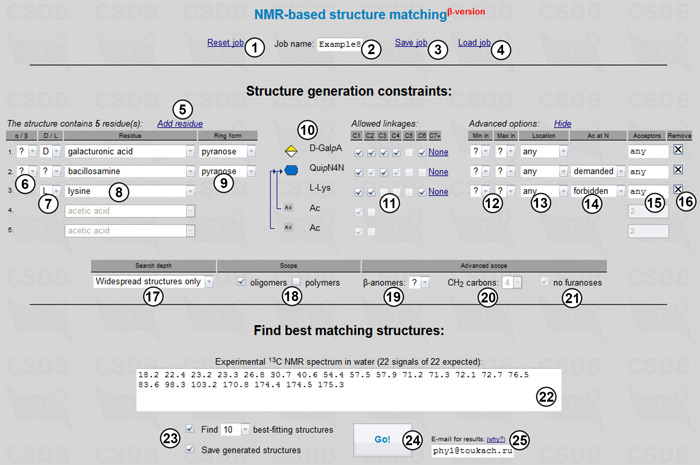 |
The tool allows resetting (1), saving (3) and loading (4) a job with the name starting with specified characters (2) from a job list. Structure generation constraints are used to define the scope of the target structures. Links (5) and (16) allows adding or removing residues. The number of rows in the table reflect the number of residues (five in our case, including acetic acid). Every row has a residue name selector (8), allowing the selection of certain residues or superclasses or ANY residue. This drop-down list contains only the most common residues; if a residue of interest is missing, it can be selected from the first entry (Show all residues). Depending on the selected residue, the section contains the following fields where applicable: anomeric configuration (6); absolute configuration (7); and residue ring form (9). Each of these fields can remain undefined (question mark). If a certain residue is known to have multiple instances in the structure, it should be specified several times. An overview of the specified limitations on the monomeric composition is presented in preview area (10).
Checkboxes in the Allowed linkages area (11) indicate which positions in each residue can be substituted during structural permutations. Only chemically possible structures will be generated, implying the inter-residue bonds can only be formed with elimination of water or ammonia. For large sugars, C7+ relates to any carbon positions higher than C6. The outgoing linkage position (usually C1 in aldo-sugars or C2 in keto-sugars) should also be checked unless a residue is at the reducing end. The Min and Max drop-down lists (12) define the minimal and maximal number of substituents that can be attached to the residue, except glycosidic bond acceptors. The default value any means no limitations, whereas - (hyphen) means that a residue can be in the terminal position only. Location (13) restrains the location of the residue in a structure. It can be any, terminal, reducing, and any except reducing. The N-acetylation drop-down list (14) defines whether amino groups of the residue are acetylated (demanded) or free (forbidden); allowed means that both variants are possible. As soon as demanded was selected for bacillosamine, two acetic acid residues were added automatically, and amino-bearing positions in bacillosamine were pre-checked in the linkage area (11). Acceptors of every residue (15) allow the specification of partial structures, if known. The list of acceptors uses residue order numbers, which you can find in the beginning of each row, and partial structures are visualized by blue arrows in the preview area (10).
Although we do not know absolute configurations, we assume they fit those occurring naturally. These common values will be used automatically in Widespread mode (17), which also excludes rarely-occurring structural features, such as atypical residues (if exact monomeric composition is not known) and ring sizes, ether and amide bonds between sugars, highly branched patterns, and large side chains in polymers. We usually know whether the structure is oligo- or polymeric; in this case, we will check oligomers (18) only. Other possible structural scope limitations, which can be determined from simple analysis of 1D NMR spectra, are the total number of β-anomeric residues (19), the total number of CH2 carbons (20), and postulated absence of furanoses (21). Some of these fields can be blocked at having a value corresponding to the selected residues and their configurations.
We enter the experimental 13C NMR spectrum in field (22), inputting the signals of multiple integral intensity more than once. If the number of signals does not conform to the range matching the selected monomeric composition, it is highlighted in the field header. We will use default number of top-matching structures to predict (23). Besides browser, results are delivered to e-mail specified in field (25), which can be useful if calculation takes longer than your browser timeout.
Pressing the Go! button (24) runs the structure iteration and empirical 13C NMR simulation. At the second phase best results are further refined by statistical NMR simulation. The status of calculation is continuously updated in the your browser, however you can bookmark the link to results displayed below the progress window and close the browser. When results are ready, they can be accessed using this bookmark or Load job (4) feature with your job name and the latest timestamp. Results are also e-mailed to you, and fetched to your browser if the session is still open. Depending on the constraints, the calculation may take long, e.g. calculation of hypotheses for 5-6 strictly defined residues or 2-3 unconstrained residues takes from 0.5 to 2 hours. Raw estimation of how long we have to wait for results is displayed below the progress status. In our case, calculation took about two minutes.
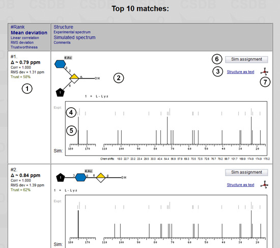 |
When the result is ready (or when you load it by clicking on the e-mailed link) it is displayed as table of structural hypotheses sorted by similarity between the simulated and the experimental NMR spectra. The first column contains the information on spectrum similarity (1): structure rank in the top-list of structural hypotheses, average deviation (shown in bold), linear correlation factor, root-mean-square deviation in ppm, and color-coded spectrum simulation trustworthiness level from 0% (red) to 100% (green) returned by the simulation engine. More details on the similarity metrics and other simulation aspects are available in the dedicated help).
The second column shows the predicted structures (2) in graphical (SNFG) or pseudographical (SweetDB) format. You can switch between these representations by clicking link (3). The experimental spectrum (in grey) (4) is aligned to the simulated one (in black) (5) for easy visual comparison. The sorted simulated chemical shifts (as well as other comments, e.g. warnings about missing signals) are listed below the spectrum. The Sim assignment button (6) runs a simulation for this structure and returns the signal assignment tables and 2D NMR spectra. A 3D icon  (7) passes the structure to the Glycoscinces.DE optimization engine, generates atomic coordinates and displays a 3D model.
Advantages and limitations of the structure elucidation algrithm, as well as expert options of the user interface are discussed in Help for GRASS - Generation, Ranking ans Assignment of Saccharide Structures.
Fragments at the termini of side chains may determine the immune response in higher organisms. Terminal residues present in the structures from human-pathogenic Aspergillus fumigatus are potential targets for probing how their presence affects the immunospecificity of strains.
The Fragment abundance link from the main menu opens the Monomer and dimer abundance tool (Fig. 9.1).
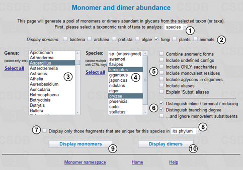 |
First we should select the target taxonomic rank, in our case - species, from drop-down list (1). We can select one or more taxa of this rank later. Other available ranks are domain, phylum, class, genus, and strain/subspecies. Since we are interested only in species from a single fungal genus, the specified display group is fungi (2). List (3) selects the genus of interest (Aspergillus) from all fungal genera present in the database. For fast navigation, we can focus on the list and start quick-typing the genus name.
When the genus is selected, a list of its species appears in field (4). This list contains only those species compounds from which are present in the database. From the list, we select two species, A. fumigatus and A. oryzae.
Checkboxes (5) and (6) define the search scope. Not checking Combine anomeric forms will treat different anomers as separate residues rather than combine them in a single entity. The Include undefined configs option allows processing of residues with undetermined anomeric, absolute or ringsize configurations, which are otherwise excluded from the statistics. We will not include them, as well as aglycons, aliases and monovalent residues (such as methyl and acetyl substituents) for clarity (5). Checkboxes (6) determine how to display the position of a residue in the structure and residue branching degree (the number of substituents, including monovalent ones; to ignore monovalent substituents, check the corresponding checkbox).
Checkbox (7) allows displaying only fragments unique for this taxon (in our case - species) as compared to all biota, its kingdom or phylum (8). Buttons (9) and (10) run statistics on monomers and dimers, correspondingly. Pressing button (9) displays the table of monomers present in glycans and glycoconjugates from A. fumigatus and A. oryzae (Fig. 9.2).
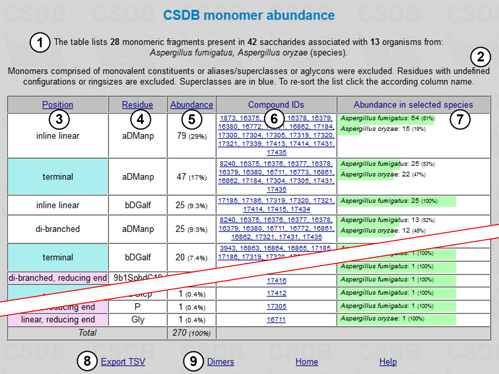 |
There is an overview stating the number of fragments, structures and organisms found (1) and the restrictions applied (2). The table of results includes the following columns: position of the residue in the structure if it was checked to be distinguished (terminal residues are shown in cyan and residues at the reducing end in pink; the branching degree is also indicated) (3); residue names and configurations (4); abundance (how many times a particular residue occurs in the structures matching the query) (5); compound IDs (links to the corresponding compounds) (6); and abundance in selected taxa (7). The page also contains accessory links, e.g. export of results to tab-separated values (can be copy-and-pasted into Microsoft Excel or other spreadsheet software) (8) and statistics on dimers for the current query (9).
According to the results, CSDB contains 42 saccharides from A. fumigatus and A. oryzae, and these saccharides are comprised of 28 monomeric residues, α-D-mannopyranose being the most abundant. The columns may be sorted by position, residue name or abundance by clicking on the column captions (3), (4), or (5). The results show that rarely occurring β-D-galactofuranose occupies the terminal position in 20 structures from A. fumigatus; thus the presence of this residue is a potential candidate for probing for the immunospecificity of A. fumigatus fungi.
This problem addresses the unique features of the genus Lupinus in terms of biosynthesis of glycans, and allows prediction of unique lupin glycosyltransferases for further search in proteomic databases.
This query can be performed using the Fragment abundance tool available from the main menu. The query form is shown in Fig. 10.1.
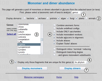 |
Here we select a taxonomic rank as genus (1) and the display group as plants (2) and then choose the Lupinus genus from the corresponding list (3). To see dimers built not only of monosaccharides but also of monovalent residues, aglycons and aliases, the corresponding checkboxes should be checked (4). If the Explain Subst aliases checkbox is unchecked, all substituents for which there are no reserved residue names in the database will be displayed as Subst and treated together. Since the study of dimeric fragments is the first step for revealing transferases, the Include undefined configs checkbox is unchecked, and the result will contain no fragments with underdetermined entities or unknown linkage positions.
To find only fragments extracted from this genus but not from any other organism belonging to the Streptophyta phylum (higher plants), we check checkbox (5) and select phylum from drop-down list (6). Pressing button (7) processes the query.
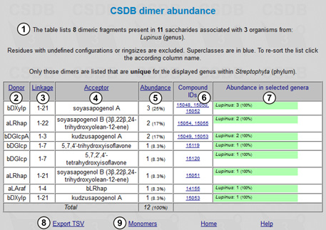 |
The resulting table is shown in Fig. 10.2. There is an overview stating the number of fragments, structures and organisms found (1). The table consists of the following columns: donor (2), linkage (3), and acceptor (4) (reflecting two residues in the dimeric fragment and the linkage between them, respectively); abundance (how many times a particular dimer occurs in the structures matching the query) (5); compound IDs (links to the corresponding compounds) (6); and abundance in selected taxa (may be less than 100% if multiple taxa were selected for comparison; in our case, there is a single taxon, Lupinus) (7). This table can be exported to tab-separated values for further processing in spreadsheet software (8). Link (9) displays the monomeric fragment statistics for the same query. We can see that there are seven lupin-specific dimers containing a characteristic aglycon moiety at the reducing end, of which 21-O-β-D-xylopyranosyl-soyasapogenol A is the most frequent. Of those compounds deposited in the database, lupins possess a single disaccharide unique in higher plants, namely 4-O-α-L-arabinofuranosyl-β-D-rhamnopyranose.
To review coverage for a particular taxonomic group(s), we select the Coverage stats link from the main menu.
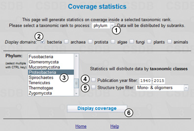 |
Fig. 11.1 shows the Coverage statistics form. Here we select a taxonomic rank, in our case - phylum (1), and the display group, bacteria (2). Then we select Proteobacteria from drop-down list (3). Publication year span (4) and structure type (5) filters are available. The Display coverage button (6) processes the query.
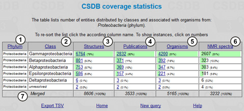 |
The results are shown in Fig. 11.2. The table includes the following columns: selected taxon(s) (1) (in our case, a single phylum was selected, so all the rows in this column are the same); subtaxa of the selected taxon(s) (2) (in our case, classes comprising the Proteobacteria phylum); structures (number of structures for the corresponding subtaxon found in the database, together with their part of the total number of structures found for the whole taxon) (3); publications (number of publications in which these structures are present) (4); organisms (number of taxonomically distinct organisms or groups of organisms from which these structures were obtained) (5); and NMR spectra (number of NMR spectra for these structures present in the database) (6). The cumulative values are shown in the last row (7).
The numbers of structures, publications and organisms are links to lists of the corresponding compounds, articles and organisms. The table can be sorted by clicking column captions (1-6).