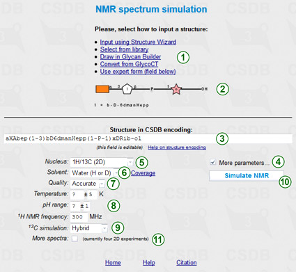
This feature is available from the NMR simulation link in Extras section of the main menu, and from the (Sub)structure search form. To simulate the NMR data, you should first enter the structure of interest. Options to do this (1) are described in the (Sub)structure search section of Usage Help. This structure is previewed in SNFG format in area (2) and copied to the structure field (3) as a term in CSDB Linear encoding. The structure can be refined by manual editing of this field.
By default, only the nucleus (5) and solvent (6) parameters are displayed, however checking More parameters... (4) shows all of them, as in the figure.
Selection of 1H/13C for nucleus (5) will simulate 1D and 2D NMR spectra (COSY, TOCSY, edHSQC, and HMBC) for both nuclei.
Solvent selector (6) restricts simulation to data obtained in a specific solvent. Please note, that if empirical or hybrid method is selected for 13C simulation, only water or unrestricted can be selected as a solvent. CSDB contains ca. 4600 NMR spectra recorded in water (mainly of structures typical for bacteria) and ca. 1700 spectra recorded in pyridine (mainly of structures typical for plants), facilitating accurate simulation of the NMR data in these solvents. The distribution of solvents vs. records in the database can be displayed by presing Coverage link (6).
There are three modes of simulation regarding quality vs. speed: fast, accurate (default), and extreme. If you see unpredicted signals (question marks) in the assignment, set the quality option (7) to higher quality and press button (10) once again. Note that in the extreme quality mode, the calculation may take up to 15 minutes.
Together with the solvent, additional simulation parameters (8), such as pH or temperature range, allow limiting the database scope to the data obtained under certain experimental conditions. Solvent, quality mode, and additional parameters are applicable to the statistical simulation only, so they are disabled if empirical 13C simulation (9) is selected. 1H NMR frequency (8) is used together with coupling constant estimation module for raw predition of the cross-peak widths in 2D spectra.
More experiments checkbox (11) adds more NMR experiments (DQF COSY, COSY RCT, HSQC-COSY, HSQC-TOCSY, depending on the selected nuclei) to 2D plots, however calculation takes longer.
If the default option (hybrid) is selected for 13C simulation (9), both empirical and statistical simulation approaches will be employed to obtain hybrid carbon chemical shifts. The empirical simulation is based on the incremental scheme with steric correction and utilizes internal databases of reference chemical shifts of mono-, di- and trimeric fragments and substitution effects. The statistical simulation is based on sequential generalization of the atomic surrounding of the predicted atom until enough structurally similar fragments are found in CSDB, with subsequent outlier detection and data averaging. The hybrid approach combines the results of empirical and statistical simulations in accordance with trustworthiness reported by both of them. It becomes available if the solvent is water or unrestricted. Proton chemical shifts are always simulated statistically.
Pressing button (10) simulates the NMR spectra and the result is displayed below the form.
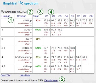
The empirical NMR simulation uses an incremental scheme to predict 13C NMR chemical shifts. Accuracy, advantages and disadvantages of this method are discussed below in this document. The empirical prediction displays a chemical shift assignment table, applied substitution effects, and subspectra of the unsubstituted residues for reference. Every row represents a certain residue in the structure of interest. Columns include:
Next to the table are the sorted spectrum as a series of chemical shifts (one atom = one value) and its graphical plot. If some signals could not be predicted, the warning displays the number of missing peaks.
The table is exportable as TSV for usage in spreadsheet software. Supplementary data (effects etc.) can be hidden for convenient copy-and-pasting.
The statistical NMR simulation uses a database-driven scheme to predict 13C and 1H NMR chemical shifts. Accuracy, advantages and disadvantages of this method are discussed below in this document. The statistical prediction displays chemical shift assignment tables, expected simulation accuracy, and links to track the origin of data.
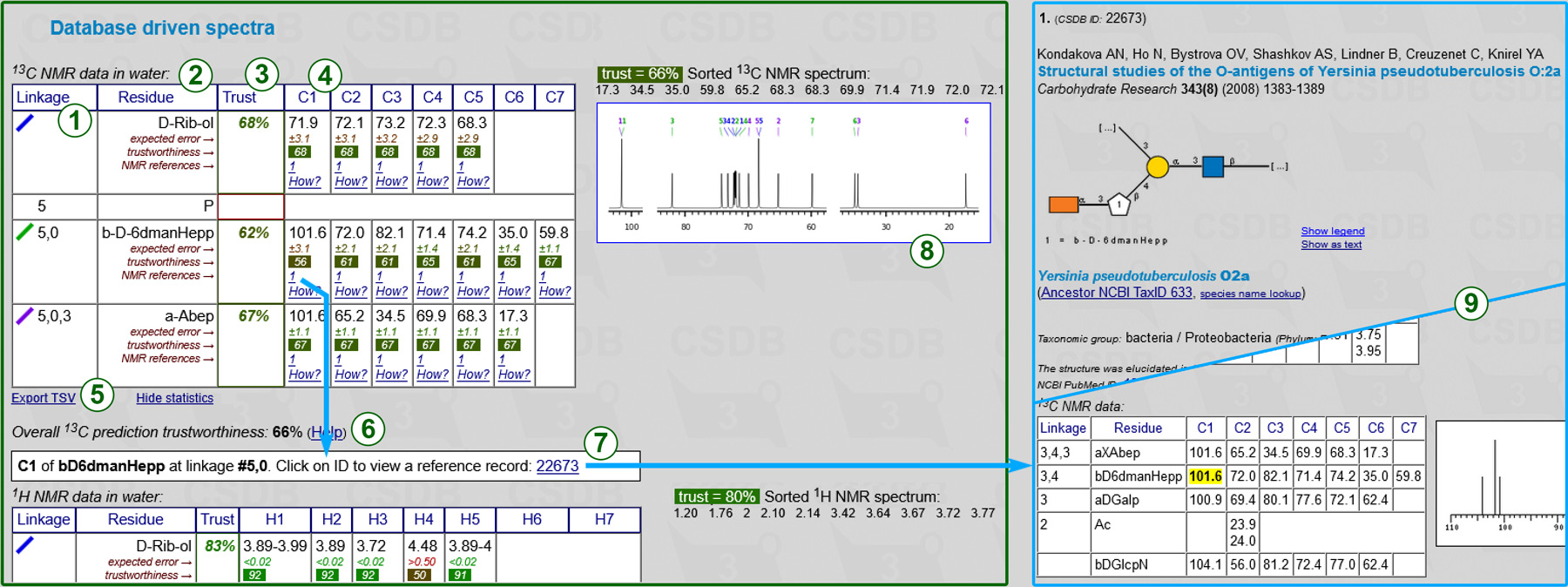
Every row represents a certain residue in the structure of interest. Columns include:
Next to the 13C assignment table are the sorted spectrum as a series of chemical shifts (one atom = one value) and its graphical plot with signal assignment (8). The assignment uses the residue color code from column (1) and atom numbering used in carbohydrate chemistry. Clicking on the spectrum opens it in a new tab in high resultion. If some signals could not be predicted, the warning displays the number of missing peaks. 1H NMR spectra are not plotted.
The table is exportable as TSV (5) for usage in spreadsheet software. Supplementary data (trustworthiness, references) can be hidden for convenient copy-and-pasting.
The hybrid carbon chemical shift simulation implies heuristic mixing of data from both approaches mentioned above according to the inter-approach deviation, trustworthiness, dataset size and other parameters. As it benefits from both simulation methods, it usually provides most accurate results. This feature is available only if both empirical and statistical simulations have been run, and the solvent in the latter approach was unrestricted or water. The hybrid prediction displays a chemical shift assignment table and the schematic superimposed NMR spectrum.
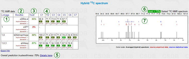
Every row represents a certain residue in the structure of interest. Columns include:
Next to the table are the sorted spectrum as a series of chemical shifts (one atom = one value) and its graphical plot. The reference data from both approaches (red marks = empirical, blue marks = statistical) are added to the spectrum plot (7). The header reports the overall trustworthiness metrics and lists all signals in sorted order (6) for copy-and-pasting. If some signals could not be predicted, the warning displays the number of missing peaks.
The table is exportable as TSV for usage in spreadsheet software.
If 1H or 1H/13C was specified as a nucleus, 2D NMR spectra are visualized using the predicted chemical shifts and rougly estimated proton coupling constants. Depending on the nucleus and the state of More NMR experiments checkbox, two to eight 2D spectra are plotted. These experiments cover most of proton and carbon spin correlations commonly used in glycobiology (COSY, TOCSY, HSQC, HMBC and derived experiments). NOE correlations are currently not supported. As an example, COSY, edHSQC and HMBC are shown in the figure (1). A quick help links ( ) beside the experiment names provide brief descriptions of what the signals in this spectrum reflect. In the edHSQC spectrum, positive cross-peaks are displayed as ellipses, while negative ones are displayed as rectangles. Links (2) lead to the derived experiments related to that displayed.
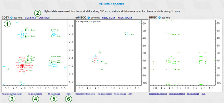
Links below the spectrum switch useful display options: color mode, signal labels and image resolution.
The color mode switch (3) determines how the signals are colored; it has two states: signal assigment and trust level. The former colors all the signals according to the residue color code, as displayed in the first column of the assignment table (exemplified in COSY and edHSQC). The latter colors all the signals in the range from red to green reflecting how accurate the simulation of the signal was (exemplified in HMBC).
The peak label switch (4) hides or shows the numbers beside signals. In the assignment color mode, these numbers correspond to the order of carbon atoms in residues. The combination of the color (=residue) and the label (=position in a residue) identifies every atom. NMR spectra, which provide non-direct correlations, may have complex labels, including bicolored ones (e.g. H1/C3) to identify inter-residue cross-peaks. In the trustworthiness color mode, numbers are the trustworthiness metrics. In the figure, HMBC is displayed without labels in the trustworthiness color mode, while COSY and edHSQC are displayed with labels in the assignment color mode.
The Hi-res image link (5) or clicking on a spectrum displays a larger image in a separate window for copy-and-pasting. If some of the signals could not be predicted (they have ? as a chemical shift in the assignment table), they are listed below the spectra in which they should have appeared.
The JDX link (6) exports the 2D spectrum in Jcamp-DX format. Two drop-down options are available:
The statistical NMR simulation is proposed for simulation of 13C and 1H chemical shifts for glycan structures, including oligomers, polymers and fragments. It outputs the NMR assignment tables, and plots 2D NMR spin correlations commonly used in glycobiology. The approach was reported as a part of Glycan-Optimized Database-Driven Empirical Spectrum Simulation (GODDESS). It has the following key features:
The used structural surrounding generalization scheme is optimized for carbohydrates and their derivatives. It was proven to provide the 13C and 1H chemical shift simulation with the accuracy outperforming the quantum mechanical methods (e.g. GIAO DFT B3LYP) in large basis sets. Root means square deviation of 0...3.0 ppm (13C) or 0...0.3 ppm (1H) depending on how many similar structural fragments have NMR spectra stored in CSDB; typical values obtained on a pool of naturally-occurring glycans were 0.9 ppm (13C) and 0.1 ppm (1H)). Besides NMR prediction, this approach is applicable to any atomic properties deposited in the database. The details are available in dedicated publications.
The trustworthiness level is estimated for every signal in the range 0..100%, the higher the better. This value is based on:
The expected prediction error (in ppm) is estimated from trustworthiness values using the linear regression. The regression rules were based on the correlations between these two parameters observed for various structure samplings.
The simulation engine searches CSDB for the fragment of a structure containing the residue with the atom under prediction, and all the adjacent residues that occupy the neighboring topological nodes. If such fragment is found, the data for the atom being predicted are checked for statistical outliers and averaged. Otherwise, the engine starts to apply generalizations of the structural surrounding from minor to major ones, until the obtained structural pattern is found in the database. Every act of generalization changes the fragment properties so that more potential structures match it. For example, a permutation of aDFucp into DFucp is a generalization act, as the former corresponds to a single fully determined fragment, while the latter matches two fragments: aDFucp and bDFucp. The figure below exemplifies some of possible generalization pathways for prediction of the C4(GlcN) chemical shift in a structure containing the aDManp(1-3)bDGlcpN(1- dissacharide fragment. Each blue arrow implies a single generalization act.
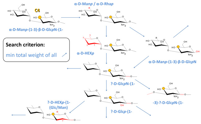
Every structural parameter of a fragment which can be generalized is assigned a weight factor depending on how strong is the expected effect of this parameter on the chemical surrounding of the analyzed atom. The estimation of this dependence empirically accounts for the nature of the parameter and its bond-distance from the predicted atom. The generalization sequence starts from parameters related to the most distal and conformationally flexible groups of atoms to minimize the effect of a generalization act on the predicted atom.
The generalizable descriptors are the following (term residue refers to a residue the predicted atom belongs to):
The weight factors were optimized iteratively to give the minimal deviation between the predicted and the experimental chemical shifts in a training set of structures. Every weight factor in a set lies in the range of 0..100 and depends on the following parameters:
The three quality vs. speed modes are supported. The logics underlying these modes is the following:
The incremental NMR simulation is proposed for the prediction of 13C chemical shifts in water solution for glycan structures, including oligomers, polymers and fragments. This approach was adapted from Biopolymer Structure Elucidation (BIOPSEL) software reported earlier. It has the following key features:
The used empirical scheme was proven to provide better accuracy than quantum-chemical methods that were usually considered the best for NMR chemical shift simulation in organic chemistry, e.g. COSMO+B3LYP/6-311++G(2d,2p). You can expect a root means square error from less than 0.5 ppm (if a glycan contains widespread residues highly populated in the spectroscopic databases) to 3.0 ppm (for rare and unusual glycans and glycoconjugates). See details in a review on glyco-NMR simulation [Chem Soc Rev 2013].
The hybrid approach combines results from the incremental and statistical simulations in accordance to the trustworthiness reported by both approaches. More details on the averaging rules are available below.
The accuracy of simulation is an average of accuracy values for every residue in a structure, and ranges 0 to 100%. Spectra predicted with the accuracy above 75% may be considered quite trustworthy. The simulation accuracy of each residue depends on the following:
If a spectrum of an exact structural fragment (dimer or trimer) is found, the accuracy is 100%.
Otherwise the simulator applies substitution effects to a spectrum of the unsubstituted residue, and the accuracy is calculated as 25*(3.5-max(EffP)-Prox), where
EffP is a perturbation introduced by the effect application (worst among all effects applied, see below),
Prox is a proximity term summed over all effect pairs (1.0 if two effects were applied on neighboring carbons, 0.5 if two effects were applied on carbons two bonds away from each other).
The effect perturbation term (0 = best, 3 = worst) may have the following values depending on which chemical shift increments were found in the theoretical effect database:
The used structural descriptors and default increments are listed in the next section.
The primary spectroscopic database and the substitution effect database contain averaged literature data on chemical shifts, glycosylation and phosphorylation effects. The approximate coverage is 80 residues, 2500 dimers and trimers, and 150 theoretical effects; data are averaged for D2O solutions at 318K. The following structural peculiarities are taken into account when searching for particular chemical shifts or substitution effects:
The simulator iterates through all residues in a structure and searches the primary spectroscopic database for chemical shifts characteristic for this residue in given structural enclosement. If these data are not found, a subspectrum of the residue is calculated from the spectrum of the unsubstituted residue and substitution effects.
If the desired effect is missing from the database, the type and orientation of a substituent next to the bonding atom in the donor residue are perturbed until the effect is found. If the perturbed effect is not found, the residue under prediction is temporarily replaced with a more widespread residue with the same basic configuration (e.g. Gal instead of FucNAc). If still no effect is found, it is simulated using the default increments.
The default increments are:
If a residue subspectrum is calculated using substitution effects (rather than extracting the exact chemical shifts from the database), chemical shifts of C2 and C5 of non-reducing pyranoses are modified the following way:
Glycosylation effects for three widespread sugar configurations (glc, gal, man) are represented most fully, usually making the effect prediction for these basetypes more accurate. The chemical shift database contains limited data on non-N-acetylated aminosugars; thus, you should virtually N-acetylate them for better accuracy.
The hybridized spectrum benefits from combining the incremental and the database-driven predictions. The spectrum averaging algorithm uses the following parameters from the empirical (emp) and statistical (stat) simulations of every signal:
In calculation of the averaged chemical shift, three options are possible:
The details on how these formulas were obtained are available in dedicated publications [J Chem Inf Model 2014, Analyt Chem 2015].
The empirical 13C NMR simulation feature was developed on the ground of the ideas of the BIOPSEL spectrum simulation software [1,2]. Within the CSDB project [8], it was adapted to oligomeric structures, was improved to treat keto-sugars and other 'special cases' and got more accurate incrementation algorithm and web-interface. This and other glycan NMR simulation schemes were reviewed [3]. The statistical NMR simulation feature is based on the GODDESS [6] carbohydrate generalization scheme [4,5]. The GRASS service [7] allows semi-automated NMR-based strucural elucidation and structural hypotheses ranking.
Please cite using the following template for Experimental part in your paper (leave or remove the 2nd sentence, depending on how you used the tool):
NMR spectrum assignment was done with the help of the chemical shift reference collection and the GODDESS simulation tool for 13C [4], 1H [5], and 2D [6] NMR data at the Carbohydrate Structure Database (CSDB) portal [8,9]. To refine a set of structural hypotheses, the CSDB structural ranking tool (GRASS [7]) was used.
This tool aims at helping in structural elucidation studies and NMR spectrum assignment. It uses GRASS algorithm, which stands for Generation, Ranking and Assignment of Saccharide Structures. The tool ranks structural hypotheses according to the fit between the simulated and experimental NMR spectra. To do that, it iterates through all possible carbohydrates and their derivatives limited by specified constraints. For each generated structure, an empirical 13C NMR spectrum is simulated (see details above) and is compared to the provided experimental data. Not more than 500 best fitting structures are further refined using statistical 2D 1H,13C-HSQC (default) or 1D 13C NMR spectrum simulations (see details above), to give a few top-matching structures. These structures are displayed as best matches together with the simulated NMR data.
The iterator permutates the following structural parameters:
Permutation of ALL of these parameters may produce billions of structures, dropping the performance and negotiating the valuability of ranking. The suggested usage of this tool implies specification of as many knowns as possible; this allows for good predictional power of the remaining unknowns. For example, it can deduce anomeric configurations and residue sequence, when exact monomeric composition and linkage positions are provided. Or it can deduce linkage positions and a sequence, when a monomeric composition and configurations are provided. However, please do not expect a miracle if you provide no exact monomeric composition or none of the above-listed parameters for structures larger than tetrasaccharides.
To improve the credibility of results and make calculation faster, you can apply structural constraints obtained from the other experiments:
In most cases, natural compounds do not contain exotic features, such as rarely-occuring residues or atypical configurations, highly dendrite branching patterns or huge side chains in polymers. To exclude such structures from iteration, there is a search scope option Widespread structures only selected by default. You can uncheck this option to generate all the structures, including those unlikely to occur in nature (this will produce from ten- to hundred-fold increase in the total number of structures and calculation time). Widespread mode applies the following limitations:
Predicted structures are ranked according to the similarity of the experimental vs. simulated NMR spectrum (mean absolute distance between pairwise-matched signals, also designated as Δ). Other metrics of the goodness of fit are also reported: RMS deviation along 1H and 133C axii, linear correlation factor, and trustworthiness reported by the the simulation engine. A few structural parameters exist, which do not significantly affect the NMR observables in sacharides. If such parameters are permutated, the resulting structural variants will occupy the neighboring positions in the result list, and their metrics will be close each to other. In this case you are expected to use common sense or additional experiments to distinguish a proper variant.
The experimental NMR spectrum is allowed to have false signals or missing signals, although the bigger is the difference between the expected and provided number of signals, the less accurate results are and the longer is calculation. In this case deviation between spectra is calculated after worst-fitting signals are removed from the bigger spectrum. Every such removal (as well as every unpredicted signal in the simulated spectrum) adds a negative impact to the resulting metric.
If there are many unknowns, the calculation can take long time. You can close your browser, but calculation will go on in background, and you will be notified by e-mail when results are ready. Alternatively you can periodically check the link to the job you have started, or wait for the results in your browser. If your browser session is closed by timeout, the calculation does not stop, and you can use the provided link to access your results. Besides prediction results, logs of the generated structures and calculation errors are available.
The structure iterator and ranking scheme were developed by Roman Kapaev and Philip Toukach within the CSDB project. On usage, please cite this publication: R.R. Kapaev, Ph.V. Toukach "GRASS: semi-automated NMR-based structure elucidation of saccharides" (Bioinformatics 2018, 34(6): 957-963. DOI: 10.1093/bioinformatics/btx696).
Advantages of GRASS as compared to other solutions:
Limitations of GRASS:
In 2015, GRASS prediction power and performance have been tested on a set of 556 structures with published 13C NMR spectra recorded in water and possessing various types of structural features met in glycobiological research. A newer publication emphasizing the advantages of 2D HSQC mode, is expected in 2026. For 1D tests, if a 13C NMR spectrum of a structure was stored in CSDB, it was virtually removed from the database to avoid the statistical NMR prediction bias. The prediction power was validated in eight modes differing in knowns/unknowns combinations. The figure displays the percentage of hits when correct structure was reported in the list of top-N hypotheses predicted by 1D GRASS:
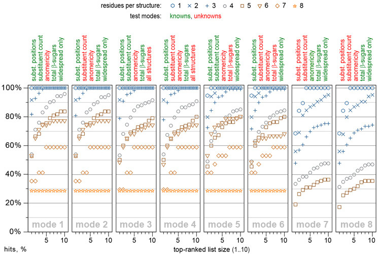
As an example, mode 1 implies specification of polymericity, monomeric composition, and total number of β-sugars per structure unit; it implies specification of allowed substitution positions, number of substituents, and N-acetylation type (allowed/forbidden/demanded) for each residue. Other parameters are unrestricted by default. In this mode, GRASS provides fair predictions of structural parameters, which are most diffucult to determine without full NMR assignment, namely the sequence of residues and their anomeric configurations. For relatively complex structures having five or six residues, correct answers were among top five matches in ~75% cases. The prediction power in most complicated cases (seven or more residues) lies within 60%, however, it can be enhanced by adding more structural constraints.
There is no substantial accuracy decrease if a total number of β-sugars and/or number of substituents per residue are not constrained. However, for structures bigger than a trisaccharide, it is very desirable to restrict allowed substitution positions retrieved from the methylation analysis. Providing no structural constraints except the number of residues is reasonable for structures with one or two residues.
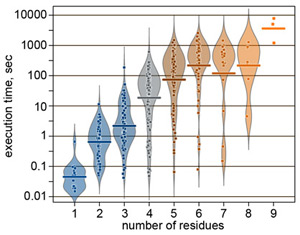
Most of the problems actual in natural carbohydrate research take from several minutes to one hour for calculation. As an example, performance in mode 1 is statistically summarized in the figure on the right.
The simplest way to use GRASS is to press Add residue as many times as the number of residues in a structure, select residues from drop-down lists, paste the HSQC chemical shifts along with 13C chemical shifts of unprotonated carbons, press the Go! button, and read the best-fitting structure under position #1 in the result list. Click here to view a screenshot with calculation of a polymer containing one glucuronic acid residue and one fucose residue per repeat unit. The screenshots were made with advanced options hidden. To uncover expert settings, click More options.... The details of GRASS user interface are discussed below.
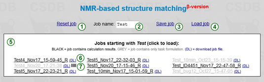
The upper part of the screen contains job management tools. The Reset (1) link resets the iterator and predictor to the default state.
The prefix field (2) allows filtering out the jobs entitled with this prefix. The default prefix is MyJob.
The Load (4) link displays the list of recent jobs (5) with names beginning with the specified prefix. The jobs are kept on the server for a month, so please download and backup your job files to save them permanently. Click on a job file in the list to load a job. The jobs displayed in grey contain only task formulation data but no calculation results. Those containing results are displayed in black and are decorated with the R character. The DL link (6) downloads a flat job file. If you see a progress indicator  (7) it means that a corresponding job is currently running. Clicking on this indicator invokes a password-protected job termination dialog. If you load an active job, the progress status will start updating (see below) and browser will wait for the results.
The Save (3) link saves a current job (including results, if present) on the server. The job name is made of a prefix specified in (2) and current date and time. Every time you (re)start the calculation, a new timestamp is used, and the job is saved automatically. If you save your job while previous calculation is still running in your browser session, the session is closed and you start over with another timestamp. However, the previously started job continues running in the background, and you can load it using Load job or the result link provided.
Pressing the Go! button starts the calculation of your job. When the calculation is finished, the results are saved to a file. A link to this file is provided when the calculation is started (4). If the browser session is still open, results are also delivered to the browser. If you close the browser, the calculation goes on in background and results are e-mailed to you when they are ready. The result link is persistent upon session close, so you can use it in future to access your results. Please keep in mind that if you close or reload the page, or save another instance of your job, this link will not be displayed anymore. So for long calculations, if you did not provide your e-mail, it is a good idea to save this link to be able to load the job results in the future.
To prevent overloading the server by concurrent tasks started from multiple pressing Go!, the button is blocked during the calculation. When the results are obtained and fetched to the browser, the button is unblocked. You can save the job and load it again to unblock the Go! button earlier; in this case your previous job will continue running in the background.
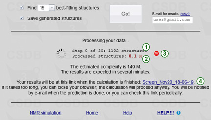
During the calculation, its progress is displayed. The first phase includes up to 400 steps, for each of which the number of generated structures is reported (1). If some of these structures failed to be processed (e.g. due to the presence of exotic structural features unsupported by the empirical simulation engine), this number is shown in the form X of Y structures, where Y structures were generated, but only X of them could be processed. The total number of generated structures is reported below (2). The second phase consists of refining up to 500 best-fitting structures by the statitical simulation and forming a few top matches.
By pressing a stop sign  (3) you can terminate the current job and release your IP adress for your other jobs. However, if you save the job (it creates a new timestamp), or load another job, or close the browser, the STOP sign will not be available anymore, and you will not be able to abort calculation of your job, although you can see which jobs are running in the Load job dialog. When requested to stop, a temporary new window displays a confirmation of job abortion, or a error message.
The raw estimation of how long you have to wait for results is displayed below the process status. If your job complexity estimation exceeds twelve hours, you are not allowed to run the calculation for free. To overcome this limitation, reduce the amount of unknowns in your task (apply more structural constraints), or register your e-mail as a priority user for 30$ (once per lifetime). Regular users can run up to two simultaneous jobs (for no longer than 12 hours each). Priority users, identified by e-mail and client IP address, can run up to four simultaneous jobs for no longer than five days each.
Below the job tools you are supposed to input the Structure generation constraints and calculation options (see the screenshot below). You can display less options if you click on Hide (2). Some fields in this form can be changed implicitly, as a reaction to the user input in the other fields. Every time it happens, as well as when user input is considered non-optimal, a warning sign  appears near a field that requires attention. Clicking on this sign displays an explanation why this warning was raised. To avoid unexpected results, it is recommended to check all warnings before starting the calculation.
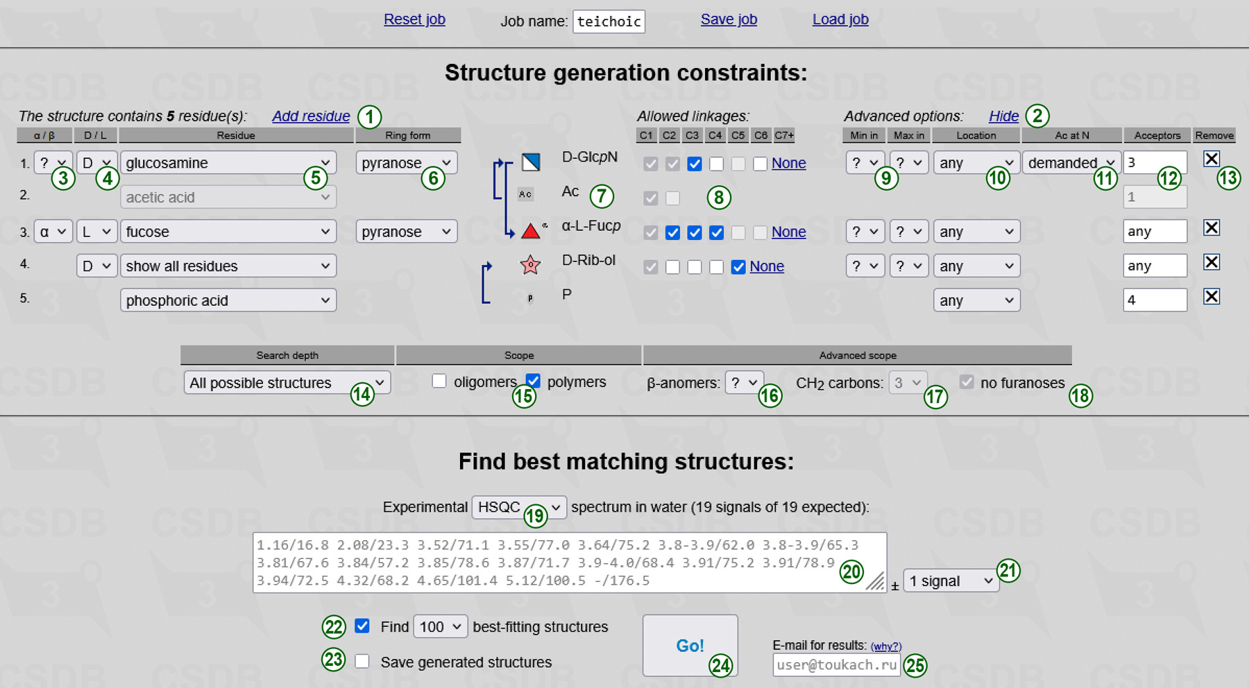
The only obligatory and non-iterated parameter is a number of residues in an oligomeric structure or in a polymer repeating unit. The default form has only one residue. You can add residues by clicking Add residue link (1), and remove them by clicking a cross sign  (13) at the right of the corresponding row. If a certain residue is present in your structure more than once, add it several times. Please note that monovalent substituents attached with elimination of water (such as acetic acid or methanol), are always considered as distinct residues, regardless to whether they are a part of OAc, NAc or other group. Every row in the form provides constraints on a single residue (identified by an order number in the beginning of the row):
(13) at the end of the row removes a residue from monomeric composition. It is shown if there are two or more residues, excluding demanded N-acetyl groups. When you remove a residue, the order numbers of the remaning residues change, and if specific connections between residues were specified, they are recalculated accordingly. Removal of a residue with demanded N-acetate removes the connected acetic acid residue as well. To remove the connected N-acetate you should first disconnect it, or select forbidden as N-acetylation state of the acceptor residue.
For your reference, the summary of a residue, including its name with all configurations applied and an SNFG icon, is displayed in the preview area (7). If partial substructures were specified, they are represented by arrows connecting the residues. More than one outgoing arrow means that a residue can have any of the depicted acceptors. No outgoing arrows mean no limitations.
The table below residue constraints (search depth and scope) allows refining the structure iteration by providing structure-wide parameters:
To Find best matching structures you are expected to input the unassigned experimental NMR spectrum recorded in water (20). Following the selector (19), the ranker can utilize either 1D 13C NMR spectrum or 2D 1H,13C HSQC spectrum (default). All generated structures are matched against this spectrum. After peak picking, type or paste space- or newline-separated chemical shifts in arbitrary order. One (for 13C) or two (for 1H) digits after a decimal dot is enough. For coincided signals of multiple integral intensity, input them more than once. Please do not forget signals of acetates and quaternary carbons, even in the 2D HSQC mode (e.g. 175/-, see below). Adding all unprotonated carbons to an HSQC spectrum will significantly increase the predictive power. If quarternary carbon peaks are too small to pick, you can use 175 for every carbonyl carbon, which you suggest to exist in your structure (e.g. a confirmed acetyl group).
In 2D HSQC mode, please pay attention to the following issues:
The expected number of signals depends on the specified monomeric composition; it can be a range if there are superclasses having a variative number of carbon atoms. This range is displayed above the spectrum together with the current number of signals, which is highlighted in red if it does not conform to the expected limits. The maximal difference between the number of signals in the experimental and the simulated spectrum (21) defaults to 1 signal. If you select no signals you should specify exactly all signals, and structures having a different number of non-equivalent carbons are filtered out. Selection of greater maximal difference (1 or 2 signals) allows skipping true signals or adding false signals in the experimental spectrum, and thus introduces tolerance to peak picking errors and allows broader interpretation of superclasses. However, this decreases accuracy and slows down the calculation.
Two flow-control options include:
Complex job calculation can take longer than your browser timeout, but it continues running in the background after the session ends. You will be notified on the e-mail you entered (25) when the results are ready, and the link to load the results will be provided. If you skip inputting the e-mail address, you do not get notified, but you can periodically check the link displayed after you pressed the Go! button (24). If you are a priority user, you must specify the e-mail address to get recognized by a combination of your e-mail and IP address.
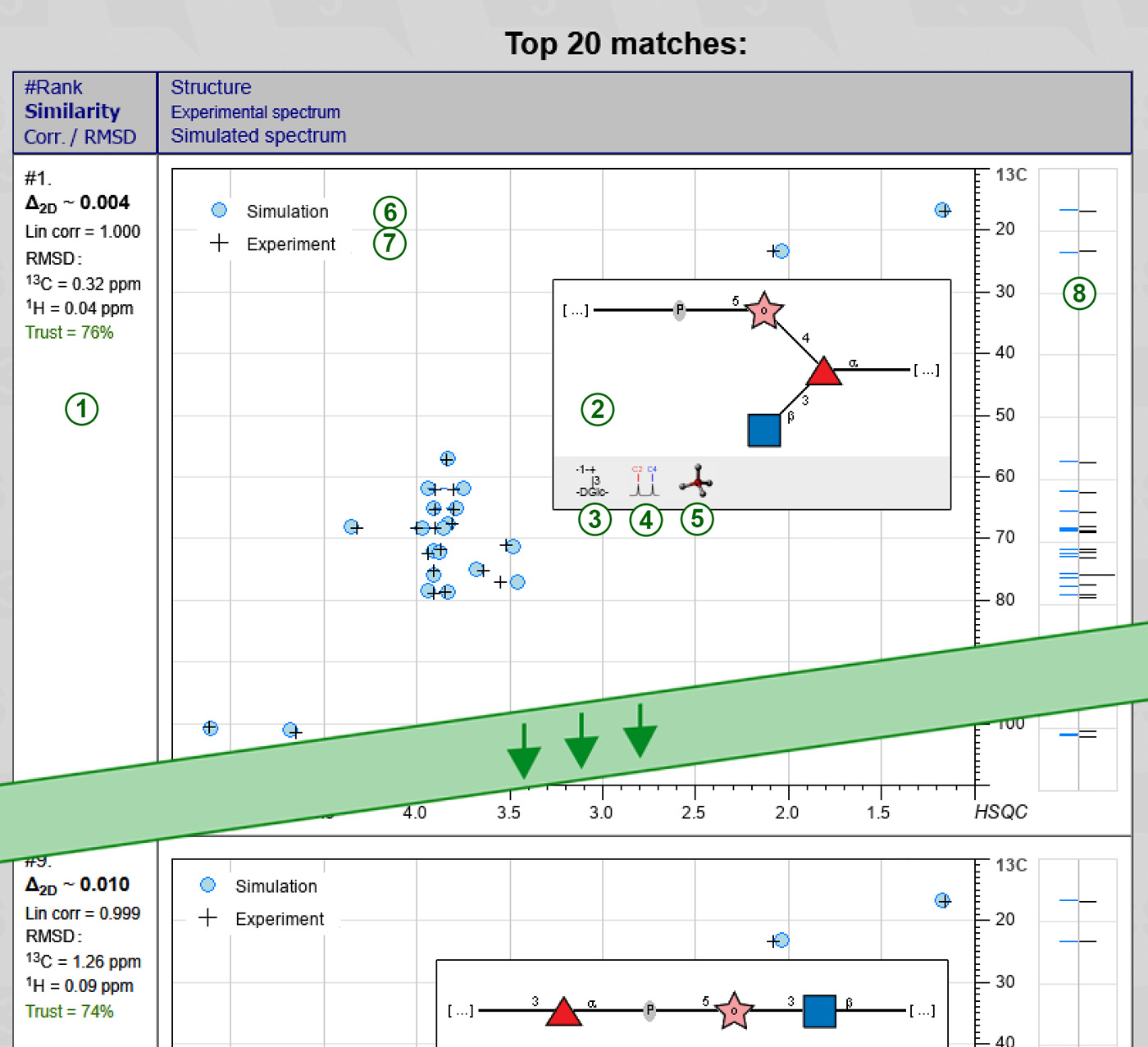
As soon as calculation is finished, the results are saved on the server, and page is reloaded to display them in a table containing the desired number of best-matching structures, one compound per row. The rows are sorted according to the deviation between experimental and simulated NMR spectra.
The left column of the result table displays metrics reflecting how good a structure in this row fits the experimental spectrum. It has several lines (1):
The second (big) column shows the predicted structure (structural hypothesis) in SNFG graphic format (2). You can switch between SNFG ( , graphic) and SweetDB (
 , pseudographic) representations by clicking on a Format toggler icon (3). Holding a mouse cursor over a graphical structure pops up a balloon with CSDB linear code of this structure.
The Sim assignment icon  (4) opens a separate window, where a predicted structure is passed to the NMR simulation module. As a result, you get assigned 13C and 1H spectra, results from three simulation methods (empirical, statistical, and hybrid), expected accuracy and trustworhiness on per-atom basis, and plotted 1D and 2D NMR spectra based on chemical shift simulation and raw estimation of coupling constants. Signal assignment in the plots and tables use a residue color code and standard carbohydrate atom numbering. Further you can export the simulated 2D spectra to process them externally and compare to the experimental ones.
Clicking on the 3D icon  (5) opens an atomic model of the structural hypothesis presented as a structural formula. Further you can click Show 3D to show an optimized most favorable conformation, download atomic coordinates in MOL or PDB format, or visually explore the model to estimate NOEs.
In 2D mode, schematical statistically simulated (6) vs. experimental + (7) HSQC spectra are superimposed in one plot. On the right, mirrored 1D 13C NMR spectra (black for experimental, blue for simulated) are shown (8). This 1D spectra can have more signals than HSQC spectra, because they contain signals of unprotonated carbons as well. However, the spectra are cropped according to HSQC bounds containing cross-peaks. To show the HSQC superimposition in high resolution, along with full 1D spectra (including, e.g. quarternery carbons at ~175 ppm), click anywhere in the plot.
In 1D mode, the statistically simulated 13C NMR spectrum is schematically plotted in black. The line height depends on the number of overlapped signals only. These multiple-intensity signals have a small horizontal line at their lower end, indicating the range from which coincided signals were gathered. The experimental spectrum is displayed in grey above the simulated one for reference. Both spectra are aligned against the same scale for easy visual comparison.
The sorted simulated chemical shifts (and other comments, e.g. warnings about missing signals) are listed below the spectrum for copy-and-pasting. If you need chemical shifts in the order of assignment to residues and atoms, press the Sim assignment icon and use the export TSV feature.
Below the table you find a copy of link to load the task and its calculation results, and links to show structure and error logs.
Clicking on Show structure log displays a report on structure generation. It contains the number of steps at phase 1, the number structures generated at each step, and the number of structures refined in phase 2. The number of structures for which empirical simulation failed to run (e.g., due to the presence of exotic reasidues) is also included. Clicking the link once again hides the structure log. If you checked option Save generated structures, all generated structures are also saved to this log in CSDB linear format. The prefix failed means that a structure could not be processed, and thus it is a priori missing from the results. For complex tasks, there can be millions of structures in this log, so if you ordered to save generated structures, please be patient while your browser opens the log.
Clicking on Show error log displays the error log. Except error messages, explaining why a certain structure could not be processed, it contains memory and performance data. Clicking the link once again hides the error log.
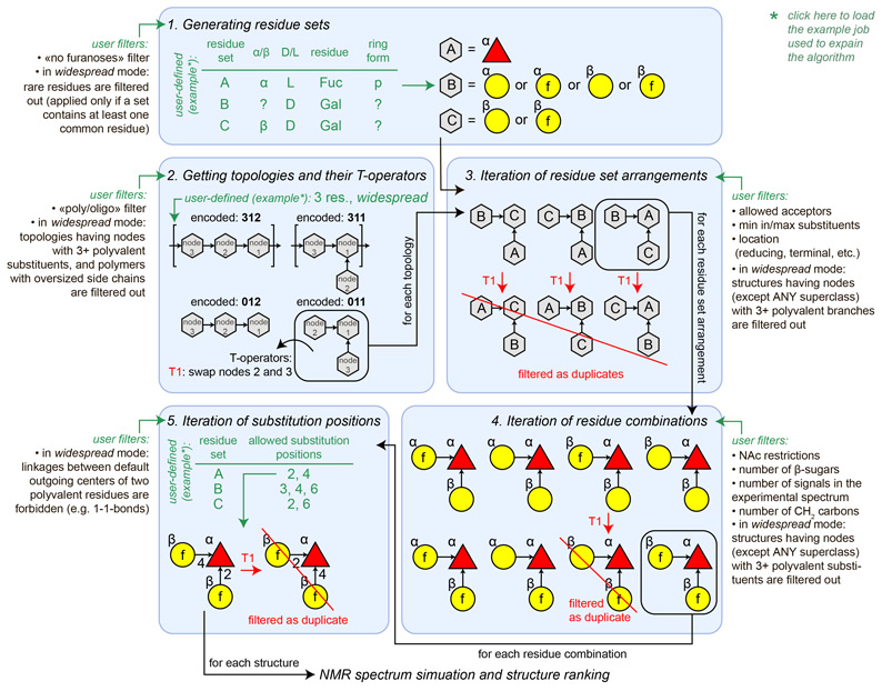
1. The structure iteration begins with processing user-defined residue names, anomeric and absolute configurations, and ring forms. For each node of structure composition, a set of candidate residues is generated basing on these constraints. For example, if residue is rhamnose, anomeric configuration (α/β) is undefined (?), absolute configuration is D, and the ring form is pyranose, the set for this residue will contain two instances, α- and β-D-rhamnopyranose. If no furanoses option is set, the resulting residue sets will lack residues in furanose form. In the widespread mode, only common residues will be included in the residue sets where possible. For example, if residue name is glucose, anomeric configuration is α, absolute configuration is ?, and the ring form is ?, the resulting residue set will include only α-D-glucopyranose; however, both D- and L- forms of α-glucofuranose will be generated if the ring form is explicitly set to furanose (for which no widespread residues are possible).
2. The next step is obtaining a list of appropriate structure topologies having a given number of residues. A topology is a directed graph, which represents how residues are linked with each other, ignoring the nature of residues. All residues are considered as identical objects (nodes), which may have one or no outgoing linkages (acceptors) and up to four ingoing linkages (substituents). To explore topologies in graphic form, click here.
Here and below, we represent topologies as strings of digits (in bold). Within the strings, the digit position (starting from 1 at the left of string) is the node order, and the digit itself stands for the order of a node it donates to. If a node has no outgoing bonds (reducing end), its digit is zero. Here are several examples of the encoded topologies:
At this stage, the total number of residues, the structural scope (polymers/oligomers), the search depth (widespread or all possible structures) and the number of terminal residues are taken into account. In the widespread mode, topologies are sorted out if they a priori meet at least one of the following criteria:
For each topology that passed through these filters, a set of all possible transposition operators (T-operators) is derived. A T-operator defines a transposition (of nodes within topology), which does not affect any structure having this topology. For example, structure aDGalp(1-4)[bDManp(1-3)]bDGlcp, which has topology 011, does not change if node 2 (galactose) and node 3 (mannose) are swapped, and substitution positions are swapped accordingly. Hence, there is a T-operator for 011, standing for exchanging nodes 2 and 3.
3. For each topology matching the constraints, all possible combinations of residue set arrangements (RSAs) are generated. Duplicate arrangements are filtered out by applying T-operators to each new arrangement and checking whether it has already been generated. At this stage, allowed acceptors, allowed locations (reducing end, terminal, etc.) and minimal/maximal numbers of substituents for each residue are taken into account. In most cases, when all residue sets include residues of the same valency (it is true for any residue name except ANY superclass), RSAs in the widespread mode are sorted out if they contain a residue with three or more non-monovalent substituents.
4. For each RSA, all combinations of particular residues are generated. Duplicate instances are filtered out by applying T-operators. Here, user-defined N-acetylation patterns (allowed,demanded or forbidden linkage of acetic acid residues to amino groups), the total number of β-sugars, a total number of signals in the experimental spectrum (total number of non-equivalent carbons), and the total number of CH2 carbons are utilized for structure filtering. The resulting combinations, which have residues with three or more non-monovalent substituents are sorted out in case they have not been exluded during step 3.
5. For each combination of residues, all possible combinations of substitution positions are generated. Duplicate instances are filtered out by applying T-operators. The substitution positions are iterated in accordance with the user input and the chemical possibility of residues to form ester, ether or amide bonds. In the widespread mode, linkages between default outgoing centers (e.g., Glc(1-1)Glc) of two non-monovalent residues are excluded.
The above notes are summarized in the figure:
This section describes the format of the NMR data in the CSDB dump file (although in the database the spectra are stored as relational tables). You need this only if you wish to upload data to CSDB.
The NMRH and NMRC fields describe assigned 13C or 1H NMR spectra, accordingly. The subspectra of each residue should be separated by double slash (//) and have the following format:
#<residue linkage>_<residue name> <chemical shifts>.
The residue names and their linkage pathes should match the structure record (see 'Structure encoding' for details).
<Residue linkage> is a comma-separated sequence of linkage positions that leads to the residue from the root of the structure (e.g. #3,2_A for residue A in the structure A(1-2)B(1-3)C). The root is either the reducing end residue or the rightmost residue in the polymer repeating unit. The linkage of the root residue is always #. Each linkage position is a number of the corresponding carbon or zero if there is no such number (e.g. for phosphoric acid residues). For carbon enumeration, please refer to Monomeric namespace subdatabase. If the linkage is unknown, use question mark (?), as in the structure record. To build the linkage through fuzzy residues, use variants with smaller substitution positions (e.g. #2,4_A but not #2,6_A in the structure A(1-2)<B(1-4)|B(1-6)>C). For dually-linked residues, use the first value as a linkage (e.g. #4_A but not #6_A for the structure A(2-4:2-6)B).
<Chemical shifts> is a space-separated list of chemical shifts of this residue in the carbon atom number ascending order. To resolve ambiguities regarding signal order or eqivalent atoms, consult the atomic patterns at the Monomeric namespace subdatabase (generally, it conforms to IUPAC numbering). If a certain chemical shift is unknown, use a question mark (?). In 1H NMR spectra, there maybe more than one or no proton signals corresponding to certain carbon numbers. In this case, separate multiple values by hyphen (-) or use single hyphen if there is no signal (e.g. -COOH groups or quaternary carbons). Please note, that every carbon in the residue must have a corresponding field in the 13C or 1H NMR subspectrum (- or ? or value), unless residue signals have not been published at all (in this case, leave the subspectrum blank, e.g. #2_Ac //)
For example, the 1H NMR assignment table for -4)aLFucp(1-P-3)[Ac(1-5)]aXNeup(2- may look like this:
#4,0_aLFucp 5.01 3.80 4.30 4.25 4.70 1.21// #4_P // #5_Ac - 2.02// #_aXNeup - - 2.32-2.38 3.60 3.40 4.40 ? 3.62 3.50-3.55 // , where H7 of neuraminic acid is unassigned.
During the search for NMR signals in the database (see Usage for help on the NMR search interface), spectra are ranked according to their similarity to the search term. To calculate the similarity between two spectra, the CSDB engine forms all possible subspectra of the larger NMR spectrum with the number of signals equal to that found in the smaller spectrum, and the best-fitting subspectrum is used to calculate the similarity value. Similarity is the reverse value of the mean pairwise deviation between signals in the sorted spectra. 1 means the average difference is 1 ppm, 10 means it is 0.1 ppm, 0.1 means it is 10 ppm etc. A value of 1000 stands for full similarity (exact match of chemical shifts). Please note, that the similarity may be very high if there are only a few signals in the smaller spectrum, but they fit well. Good similarity values for carbon spectra are 1 and above; good values for proton spectra are 5 and above.
If more than one spectrum is assigned to a compound (e.g. in different conditions or in different publications), the similarity between this compound and the given spectrum is calculated as the average of similarities of all spectra assigned to it for a given nucleus.